In my last post, I simulated a discrete Linenmayer System. L-systems evolve by repeatedly applying a transformation that is a function of the current state. Continuous dynamical systems also evolve over time according to a function of the current state, but they are described with differential equations rather than a discrete transformation function.

For example, consider a pendulum subject to gravity. The pendulum’s governing equation is:

where:

We can break the second order differential equation into two first-order differential equations by defining \(s_1 = \theta\) and \(s_2 = \dot{\theta}\).

We can then find how the state \(s\) evolves over time by finding its derivate \(\dot{s}\).

I defined a Pendulum struct to index constant parameters like gravity and pendulum length, and a function Derivative that describes how the pendulum’s state changes over time. I’ve also added air friction f to make things interesting.

// Pendulum constants.
type Pendulum struct {
	g float64    // Gravity [m/s^2]
	l float64    // Length of pendulum [m]
	f float64    // Air friction coefficient [1]
}

// Pendulum derivative function.
func (p Pendulum) Derivative(s State) State {
	s_new := make(State, len(s))
	s_new[0] = s[1]
	s_new[1] = -p.g/p.l*math.Sin(s[0]) - p.f*s[1]
	return s_new
}

Now that we’ve defined the Derivative for our plant system Pendulum, we need some way to repeatedly apply the derivative function to mutate the pendulum’s state over time.

A simple appoach is to use Euler’s Method. However, Euler’s method can accumulate a large error, especially if the time step is too large. Instead, I’ve implemented one of the higher order methods: a 4th order Runge Kutta.

In the end, I ended up with this neat little API to define and simulate your own plant systems. To simulate a plant system, you simply choose an integrator, an initial state state0, the time specification ts, and the plant system.

my_sim := Simulation{
	integrator: RungeKutta4{},
	state0:     State{0, .0001},
	ts:         TimeSpec{num_steps: 100000, t_end: 100},
	plant:      Pendulum{g: 9.81, l: 1.0, m: 1, f: .1, r: Controlled{}},
}

times, states := my_sim.simulate()

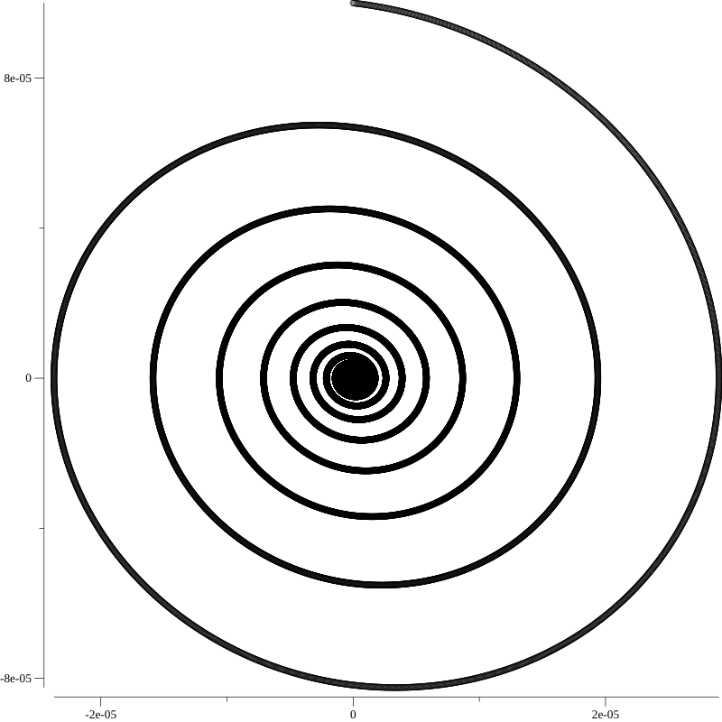
Here’s a plot of angular velocity (x) versus angular acceleration (y):

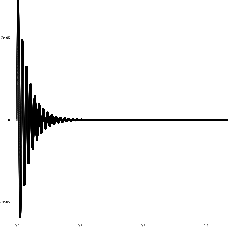
And the angular velocity over time:

The source code is here on GitHub.

Conclusion

I want to continue building out this little simulation library such that users can connect different plants and controllers to simulate larger systems. Go seems well suited to the task with its Structural Subtyping and Interfaces as first-class language constructs. Julia may also prove useful for further study.